Deep Generative Models

Understand and create complex, unstructured data.
Autoregressive Models
- Chain rule based factorization is fully general
- Compact representation via conditional independence and/or neural parameterizations
Parameterize a model family
Without loss of generality, we can use chain rule for factorization
\[p(x_1,...,x_n) = p(x_1)p(x_2|x_1) \cdots p(x_n|x_1,...,x_{n-1})\]
Fully Visible Sigmoid Belief Network (FVSBN)
The conditional variables \(X_i |X_1,···,X_{i−1}\) are Bernoulli with parameters
\[\hat{x}_i = p(X_i=1| x_1, \cdots, x_{i-1}; \bf{\alpha}^i) = p(X_i|x_{<i};\bf{\alpha}^i) = \sigma (\alpha^i_0 + \sum^{i-1}_{j=1} \alpha^i_j x_j)\]
Neural Autoregressive Density Estimation (NADE)
Improvement: Use one layer neural network instead of logistic regression.
\[\hat{x}_i = p(x_i | x_1, \cdots, x_{i-1}; A_i,c_i, \bf{\alpha}_i, b_i) = \sigma (\bf{\alpha}_i h_i + b_i)\]
Autoregressive models vs. autoencoders:
- A vanilla autoencoder is not a generative model: it does not define a distribution over x we can sample from to generate new data points.
- For autoregressive autoencoders: We need to make sure it corresponds
to a valid Bayesian Network (DAG structure), i.e., we need an
ordering.
- \(\hat{x}_1\) cannot depend on any input \(x\). Then at generation time we don’t need any input to get started.
- \(\hat{x}_2\) can only depend on \(x_1\)
Masked Autoencoder for Distribution Estimation (MADE)
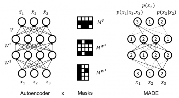
Use masks to disallow certain paths (Germain et al., 2015). Suppose ordering is \(x_2, x_3, x_1\).
- The unit producing the parameters for \(p(x_2)\) is not allowed to depend on any input. Unit for \(p(x_3|x_2)\) only on \(x_2\). And so on...
- For each unit in a hidden layer, pick a random integer \(i\) in \([1, n − 1]\). That unit is allowed to depend only on the first \(i\) inputs (according to the chosen ordering).
- Add mask to preserve this invariant: connect to all units in previous layer with smaller or equal assigned number (strictly < in final layer)
Pros & Cons
Pros
- Easy to evaluate likelihoods
- Easy to train
Cons
- Requires an ordering
- Generation is sequential
- Cannot learn features in an unsupervised way
Search for model parameters
Kullback-Leibler divergence (KL-divergence)
\[D(p||q) = \sum_x p(x) \log \frac{p(x)}{q(x)}\]
- \(D(p||q) \geq 0\) for all \(p,q\) with equality if and only if \(p = q\).
- Asymmetric, \(D(p||q) \neq D(q||p)\).
- If data comes from \(p\), but use a scheme optimized for \(q\), the divergence \(DKL(p||q)\) is the number of extra bits need on average.
Expected log-likelihood
\[D(P_{data}||P_{\theta)} = E_{x \backsim P_{data}} [ \log \frac{P_{data}(x)}{P_{\theta}(x)} ] \\ = E_{x \backsim P_{data}} [ \log P_{data}(x)] - E_{x \backsim P_{data}} [P_{\theta}(x) ]\]
The first term does not depend on \(P_{\theta}\), then minimizing KL divergence is equivalent to maximizing the expected log-likelihood
\[\arg \min_{P_{\theta}} D(P_{data} || P_{\theta}) = \arg \min_{P_{\theta}} + E_{x \backsim P_{data}} [\log P_{\theta} (x)] = \arg \max_{P_{\theta}} E_{x \backsim P_{data}} [\log P_{\theta}]\]
Empirical log-likelihood:
\[E_{\mathscr{D}} [\log P_{\theta} (x)] = \frac{1}{|\mathscr{D}|} \sum_{x \in \mathscr{D}} \log P_{\theta} (x)\]
Maximum likelihood learning:
\[\max_{P_{\theta}} \frac{1}{|\mathscr{D}|} \sum_{x \in \mathscr{D}} \log P_{\theta} (x)\]
Main idea in Monte Carlo Estimation
- Express the quantity of interest as the expected value of a random variable.
\[E_{x \backsim P} [g(x)] = \sum_x g(x) P(x)\]
- Generate T samples \(x_1, . . . , x_T\) from the distribution \(P\) with respect to which the expectation was taken.
- Estimate the expected value from the samples using:
\[\hat{g} (x^1,...,x^{T}) \triangleq \frac{1}{T} \sum^{T}_{t=1} g(x^t)\] where \(x^1,...,x^T\) are independent samples from \(P\), \(\hat{g}\) is a random variable.
Properties of the Monte Carlo Estimate
Unbiased \[E_P [\hat{g}] = E_P [g(x)]\]
Convergence \[\hat{g} = \frac{1}{T} \sum^T_{t=1} g(x^t) \rightarrow E_P [g(x)] \quad for \quad T \rightarrow \infty\]
Variance \[V_P[\hat{g}] = V_P [\frac{1}{T} \sum^T_{t=1}g(x^t)] = \frac{V_P [g(x)]}{T}\] variance of the estimator can be reduced by increasing the number of samples
Empirical Risk and Overfitting
- Empirical risk minimization can easily overfit the data
- Generalization: Model should generalize well to these “never-seen” samples.
Bias-Variance trade off:
- If the hypothesis space is very limited, it might not be able to represent \(P_{data}\), even with unlimited data (bias)
- If we select a highly expressive hypothesis class, we might
represent better the data. (variance)
- When we have small amount of data, multiple models can fit well, or even better than the true model. Moreover, small perturbations on \(\mathscr{D}\) will result in very different estimates
Avoid overfitting
- Hard constraints, e.g. by selecting a less expressive model family
- Smaller neural networks with less parameters
- Weight sharing
- Soft preference for “simpler” models: Occam Razor.
- Augment the objective function with regularization
- Evaluate generalization performance on a held-out validation set
Latent Variable Models
Mixture of Gaussians: a Shallow Latent Variable Model
Mixture of Gaussians. Bayes net: \(z \rightarrow x\).
- \(z \backsim \rm{Categorical}(1,...,K)\)
- \(p(x|z=k) = \mathscr{N}(\mu_k, \Sigma_k)\)
Generative process:
- Pick a mixture component \(k\) by sampling \(z\)
- Generate a data point by sampling from that Gaussian
Variational Autoencoder
A mixture of an infinite number of Gaussians:
- \(z \backsim \mathscr{N}(0,I)\)
- \(p(x|z) = \mathscr{N}(\mu_{\theta}(z),
\Sigma_{\theta} (z))\) where \(\mu_{\theta}, \Sigma_{\theta}\) are neural
networks
- $ _{} (z) - (Az + c) = ((a_1 z + c_1), (a_2 z + c_2)) = (_1 (z), _2 (z))$
- $ _{} (z) = \rm{diag} (((B z + d))) = $
- $ = (A,B,c,d)$
- Even though \(p(x | z)\) is simple, the marginal \(p(x)\) is very complex/flexible
隐变量z是一个多维高斯分布,\(p(x|z)\) 是一个神经网络,也是一个高斯分布。整个隐变量模型可以视为无数个高斯分布的组合,\(x\)在不同的地方对应不同的高斯分布:
\[p(x) = \int p(x|z)p(z)dz\]
MLE目标是
\[\theta \leftarrow \arg \max_{\theta} \frac{1}{N} \sum_i \log (\int p_{\theta} (x_i|z)p(z)dz)\]
上述积分不可计算,我们先把积分写成期望形式,假设 \(z \backsim p(z|x_i)\)
\[\theta \leftarrow \arg \max_{\theta} \frac{1}{N} \sum_i E_{z \backsim p(z|x_i)} [ \log p_{\theta} (x_i|z)]\]
我们不需要对所有这都计算\(p_{\theta} (x_i|z)\),只有少部分z会导致\(x_i\)的产生,这少部分z的分布为\(p(z|x_i)\),可记为\(q_i(z)\),其分布可能非常复杂(后面令其神经网络化)。 \(q_i (z)\)无法被用于精确计算\(\log p_{\theta}(x_i)\),但可求其下界,i.e., 变分推断。
Marginal Likelihood 边缘似然
概率:已知一些参数的情况下,预测接下来观测所得到的结果。
似然性:已知的某些观测所得到的结果时,对有关事物的性质的参数进行估计。
在统计学中,边缘似然函数(marginal likelihood function),或者积分似然(integrated likelihood),是一个某些参数变量边缘化的似然函数(likelihood function)。在贝叶斯统计范畴,它可以被称作为证据或者模型证据的。
Evidence Lower Bound
Log-Likelihood function for Partially Observed Data is hard to compute:
\[\log (\sum_{z \in \mathscr{Z}} p_{\theta} (\bf{x}, \bf{z})) = \log (\sum_{z \in \mathscr{Z}} \frac{q(z)}{q(z)} p_{\theta (\bf{x}, \bf{z})}) = \log (E_{z \backsim q(z)} [ \frac{p_{\theta} (\bf{x}, \bf{z})}{q(z)} ])\]
- log() is a concave function. \(\log(px + (1 − p)x^′) ≥ p \log(x) + (1 − p) log(x^′)\).
- Idea: use Jensen Inequality (for concave functions):\(\log E[y] \geq E[\log y]\):
\[\log (E_{z \backsim q(z)} [f(z)]) = \log (\sum_z q(z)f(z)) ≥ \sum_z q(z) \log f(z)\]
Choosing \(f(z)=\frac{p_{\theta}(\bf{x},\bf{z})}{q(z)}\)
\[\log (E_{z \backsim q(z)} [\frac{p_{\theta}(\bf{x}, \bf{z})}{q(z)}]) ≥ E_{z \backsim q(z)} [\log (\frac{p_{\theta (\bf{x}, \bf{z})}}{q(z)})]\] Called Evidence Lower Bound (ELBO).
Variational inference
Suppose \(q(z)\) is any probability distribution over the hidden variables, evidence lower bound (ELBO) holds for any \(q\)
\[\begin{aligned} \log p(x;\theta) &\geq \sum_z q(z) \log (\frac{p_{\theta}(\bf{x},\bf{z})}{q(z)}) \\ &= \sum_xq(z) \log p_{\theta} (\bf{x},\bf{z}) - \sum_z q(z) \log q(z) \\ &=\sum_z q(z) \log p_{\theta} (\bf{x},\bf{z}) + H(q) \end{aligned}\]
Equality holds if \(q = p(z|x;\theta)\)
\[\log p(x;\theta) = \sum_z q(z) \log p(z,x;\theta) + H(q)\]
In general, \(\log p(x;theta) = \rm{ELBO} + D_{KL} (q(z) || p(z|x;\theta))\), the closer \(q(z)\) is to the posterior \(p(z|x;\theta)\) the closer the ELBO is to the ture log-likelihood.
\[\begin{aligned} \log p(x;\theta) &\geq \sum_z q(z;\phi) \log p(z,x;\theta) + H(q(z;\phi)) \\ &= \mathscr{L}(x;\theta,\phi) + D_{KL} (q(z;\phi)|| p(z|x;\theta)) \end{aligned}\]
or
\[\begin{aligned} \mathscr{L} = E_{z \backsim q_{\phi}(z|x)} [\log p_{\theta} (x|z) + \log p(z)] + H(q_{\phi}(z|x)) \end{aligned}\]
\(\mathscr{L}(x;\theta,\phi)\)为ELBO,通过最大化ELBO将下界推高。 由于KL散度永远大于0,\(\log p(x_i)\)的值不随\(q_i (z)\)的变化而变化。当使\(q_i (z)\)逼近\(p(z|x_i)\)时,\(\mathscr{L}(x;\theta,\phi)\)能取最大值,因此我们需要最小化\(D_{KL} (q(z;\phi)|| p(z|x;\theta))\)
Normalizing Flow Models
Key idea behind flow models: Map simple distributions (easy to sample and evaluate densities) to complex distributions through an invertible transformation.
- Typically consider parameterized densities:
- Gaussian: \(X \backsim \mathscr{N} (\mu,\sigma)\) if \(p_x (x)=\frac{1}{\sigma \sqrt{2 \pi}} e^{-(x-\mu)^2 /2\sigma^2}\)
- Uniform: \(X \backsim \mathscr{U}(a,b)\) if \(p_x (x)=\frac{1}{b-a} 1[a \leq x \leq b]\)
- If \(X\) is a continuous random
vector, we can usually represent it using its joint probability
density function:
- Gaussian: if \(p_x (x) = \frac{1}{\sqrt{(2\pi)^n} |\Sigma|} \exp (-\frac{1}{2} (x - \mu )^T \Sigma^{-1} (x - \mu))\)
Change of Variables formula
Change of variables (1D case): If \(X=f(Z)\) and \(f(·)\) is monotone with inverse \(Z=f^{−1}(X)=h(X)\), then: \[p_X (x) = p_Z (h(x)) |h^{'} (x)|\] Note that the ”shape” of \(p_X(x)\) is different (more complex) from that of the prior \(p_Z(z)\). Letting \(z=h(x)=f^{−1}(x)\) we can also write \[p_X (x) = p_Z (z) \frac{1}{f^{'} (z)}\]
Generalized change of variables
- For linear transformations specified via \(A\), change in volume is given by the determinant of \(A\)
- For non-linear transformations \(f(·)\), the linearized change in volume is given by the determinant of the Jacobian of \(f(·)\)
- Change of variables (General case): The mapping between \(Z\) and \(X\), given by \(f:{\Bbb{R}}^n \mapsto \Bbb{R}^n\), is invertible such that \(X = f(Z)\) and \(Z = f^{−1}(X)\). \[p_{X}(x) = p_{Z} (f^{-1}(x)) |\det (\frac{\partial f^{-1} (x)}{\partial x})|\]
- \(x, z\) need to be continuous and have the same dimension.
- For any invertible matrix \(A\), \(\det(A^{−1}) = \det(A)^{−1}\) \[p_{X}(x) = p_{Z} (z) |\det (\frac{\partial f (z)}{\partial z})|^{-1}\]
In a normalizing flow model, the mapping between \(Z\) and \(X\), given by \(f_{\theta}:{\Bbb{R}}^n \mapsto \Bbb{R}^n\), is deterministic and invertible such that \(X= f_{\theta}(Z)\) and \(Z = f^{−1}_{\theta}(X)\). the marginal likelihood p(x) is given by \[p_{X}(x;\theta) = p_{Z} (f^{-1}_\theta(x)) |\det (\frac{\partial f_\theta^{-1} (x)}{\partial x})|\]
Normalizing: Change of variables gives a normalized density after applying an invertible transformation Flow: Invertible transformations can be composed with each other \[z_m = f^m_\theta \circ \cdots \circ f^1_\theta (z_0) = f^m_\theta (f^{m-1}_\theta (\cdots (f^1_\theta (z_0)))) \triangleq f_\theta (z_0)\]
- Start with a simple distribution for \(z_0\) (e.g., Gaussian)
- Apply a sequence of M invertible transformations to finally obtain \(x = z_M\)
- By change of variables \[p_{X}(x;\theta) = p_{Z} (f^{-1}_\theta(x)) \prod^M_{m=1} |\det (\frac{\partial ({f^m_\theta})^{-1} (z_m)}{\partial z_m})|\]
Learning and Inference
Learning via maximum likelihood over the dataset \(\mathscr{D}\) \[\max_\theta \log p_{X}(\mathscr{D};\theta) = \sum_{x \in \mathscr{D}} \log p_{Z} (f^{-1}_\theta(x)) + \log |\det (\frac{\partial f^{-1}_\theta (x)}{\partial x})|\] Exact likelihood evaluation via inverse tranformation \(x \mapsto z\) and change of variables formula Sampling via forward transformation \(z \mapsto x\) \[z \backsim p_{Z} (z) \quad x = f_{\theta} (z)\] Latent representations inferred via inverse transformation (no inference network required!) \[z = f^{-1}_{\theta} (x)\]
Computing likelihoods also requires the evaluation of determinants of n × n Jacobian matrices, where n is the data dimensionality: \(O(n^3)\) => Key idea: Choose tranformations so that the resulting Jacobian matrix has special structure. For example, the determinant of a triangular matrix is the product of the diagonal entries, i.e., an O(n) operation.
Invertible transformations with diagonal Jacobians
Nonlinear Independent Components Estimation (NICE)
- Additive coupling layers Partition the variables \(z\) into two disjoint subsets, say \(z_{1:d}\) and \(z_{d+1:n}\) for any \(1 ≤ d < n\)
- Forward mapping \(z \mapsto x\)
- \(x_{1:d} = z_{1:d}\) (identity transformation)
- \(x_{d+1:n} = z_{d+1:n} + m_\theta (z_{1:d})\) (\(m_\theta (\cdot)\) is a neural network with parameters \(\theta\), \(d\) input units, and \(n − d\) output units)
- Inverse mapping \(x \mapsto z\)
- \(z_{1:d} = x_{1:d}\) (identity transformation)
- \(z_{d+1:n} = x_{d+1:n} - m_\theta (x_{1:d})\)
- Jacobian of forward mapping \[ J = \frac{\partial x}{\partial z} \left( \begin{matrix} I_d, 0 \\ \frac{\partial x_{d+1:n}}{\partial z_{1:d}} , I_{n-d} \end{matrix} \right) \\ \det (J) = 1\]
- Volume preserving transformation since determinant is 1.
- Forward mapping \(z \mapsto x\)
- Rescaling layers
- Additive coupling layers are composed together (with arbitrary partitions of variables in each layer)
- Final layer of NICE applies a rescaling transformation
- Forward mapping \(z \mapsto x\): \[ x_i = s_i z_i\] where \(s_i > 0\) is the scaling factor for the i-th dimension.
- Inverse mapping \(x \mapsto z\): \[ z_i = \frac{x_i}{s_i}\]
- Jacobian of forward mapping: \[ J = \rm{diag} (s) \\ \det (J) = \prod^n_{i=1} s_i\]
Real-NVP: Non-volume preserving extension of NICE
- Forward mapping \(z \mapsto x\)
- \(x_{1:d} = z_{1:d}\) (identity transformation)
- \(x_{d+1:n} = z_{d+1:n} \odot \exp (\alpha_\theta (z_{1:d})) + \mu_{\theta} (z_{1:d})\)
- \(\mu_\theta (\cdot), \alpha_\theta\) are both neural network with parameters \(\theta\) \(d\) input units, and \(n − d\) output units, \(\odot\) denotes elementwise product
- Inverse mapping \(x \mapsto z\)
- \(z_{1:d} = x_{1:d}\) (identity transformation)
- \(z_{d+1:n} = (x_{d+1:n} - \mu_\theta (x_{1:d})) \odot (\exp (-\alpha_\theta (x_{1:d})))\)
- Jacobian of forward mapping \[J = \frac{\partial x}{\partial z} \left( \begin{matrix} I_d, 0 \\ \frac{\partial x_{d+1:n}}{\partial z_{1:d}} , \rm{diag}(\exp (\alpha_{\theta (z_{1:d})})) \end{matrix} \right) \\ \det (J) = \prod^n_{i=d+1} \exp (\alpha_\theta (z_{1:d})_i) = \exp (\sum^n_{i=d+1} \alpha_\theta (z_{1:d})_i)\]
- Non-volume preserving transformation in general since determinant can be less than or greater than 1
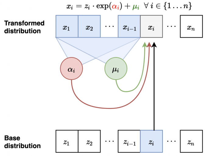
Autoregressive Models as Normalizing Flow Models
- Consider a Gaussian autoregressive model: \[ p(x) = \prod^n_{i=1} p(x_i | x_{<i})\] such that \(p(x_i|x_{<i})=\mathscr{N} (\mu_i (x_1,...,x_{i-1}), \exp (\alpha_i (x_1,...,x_{i-1}))^2)\).\(\mu_i (\cdot), \alpha_i (\cdot)\) are neural networks for \(i > 1\) and constants for \(i = 1\).
- Sampler for this model:
- Sample \(z_i \backsim \mathscr{N} (0,1)\) for \(i=1,...,n\)
- Let \(x_1 = \exp (\alpha_1) z_1 + \mu_1\). Compute \(\mu_2(x_1),\alpha_2 (x_1)\)
- Let \(x_2 = \exp (\alpha_2) z_2 + \mu_2\). Compute \(\mu_3(x_1,x_2),\alpha_3 (x_1,x_2)\)
- Let \(x_3 = \exp (\alpha_3) z_3 + \mu_3\)...
- Flow interpretation: transforms samples from the standard Gaussian \((z_1,z_2,...,z_n)\) to those generated from the model \((x_1,x_2,...,x_n)\) via invertible transformations (parameterized by \(\mu_i (\cdot), \alpha_i (\cdot)\)
Masked Autoregressive Flow (MAF)
- Forward mapping \(z \mapsto x\)
- Let \(x_1 = \exp (\alpha_1)z_1 + \mu_1\). Compute \(\mu_2(x_1), \alpha_2(x_1)\)
- Let \(x_2 = \exp (\alpha_2)z_2 + \mu_2\). Compute \(\mu_3(x_1, x_2), \alpha_3(x_1, x_2)\)
- Sampling is sequential and slow (like autoregressive): \(\mathscr{O}(n)\) time
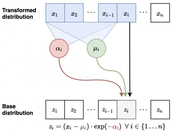
- Inverse mapping from \(x \mapsto
z\):
- Compute all \(\mu_i, \alpha_i\) (can be done in parallel)
- Let \(z_1 = (x_1 - \mu_1) / \exp (\alpha_1)\) (scale and shift)
- Let \(z_2 = (x_2 - \mu_2) / \exp (\alpha_2)\)
- Let \(z_3 = (x_3 - \mu_3) / \exp (\alpha_3)\)...
- Jacobian is lower diagonal, hence efficient determinant computation
- Likelihood evaluation is easy and parallelizable (计算\(p(x_1),p(x_2|x_1),...,p(x_D|x_{1:D-1})\)时可以并行)
- sampling autoregressive models is slow because you must wait for all previous \(x_{1:i−1}\) to be computed before computing new \(x_i\)
- Layers with different variable orderings can be stacked
Inverse Autoregressive Flow (IAF)
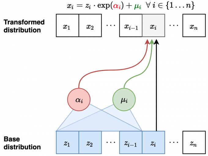
- Forward mapping \(z \mapsto x\)
(parallel):
- Sample \(z_i \backsim \mathscr{N} (0,1)\) for \(i=1,...,n\)
- Compute all \(\mu_i, \alpha_i\) (can be done in parallel)
- Let \(x_1 = \exp (\alpha_1) z_1 + \mu_1\)
- Let \(x_2 = \exp (\alpha_2) z_2 + \mu_2\)...
- Inverse mapping from \(x \mapsto
z\) (sequential):
- Let \(z_1 = (x_1 − \mu_1)/ \exp (\alpha_1)\). Compute \(\mu_2(z_1), \alpha_2(z_1)\)
- Let \(z_2 = (x_2 − \mu_2)/ \exp (\alpha_2)\). Compute \(\mu_3(z_1,z_2), \alpha_3(z_1,z_2)\)
- Fast to sample from, slow to evaluate likelihoods of data points (train)
- Note: Fast to evaluate likelihoods of a generated point (cache \(z_1,z_2,..., z_n\))
IAF vs. MAF
- Computational tradeoffs
- MAF: Fast likelihood evaluation, slow sampling
- IAF: Fast sampling, slow likelihood evaluation
- MAF more suited for training based on MLE, density estimation
- IAF more suited for real-time generation
Energy-Based Models (EBMs)
Parameterizing probability distributions
- non-negative: \(p(x) \geq 0\)
- \(g_\theta (\bf{x}) =f_\theta(\bf{x})^2\)
- \(g_\theta (\bf{x}) =\exp (f_\theta(\bf{x}))\)
- \(g_\theta (\bf{x}) =| f_\theta(\bf{x})|\)
- \(g_\theta (\bf{x}) = \log(1 + \exp ( f_\theta(\bf{x})))\)
- sum-to-one: \(\sum_x p(x) = 1\) (or \(\int p(x) dx = 1\) for continuous variables) \[p_\theta (\bf{x}) = \frac{1}{\rm{Volume} (g_\theta)} g_\theta (\bf{x}) = \frac{1}{\int g_\theta (\bf{x}) d\bf{x}} g_\theta (\bf{x})\]
- Example: choose \(g_\theta(\bf{x})\) so that we know the
volume analytically as a function of \(\theta\).
- \(g_{(\mu, \sigma)} (x) = e^{-\frac{(x-\mu)^2}{2\sigma^2}}\). Volume: \(\int e^{-\frac{x-\mu}{2\sigma^2}}dx=\sqrt{2 \pi \sigma^2}\). (Gaussian)
- \(g_\lambda (x) = e^{-\lambda x}\). Volume: \(\int^{+ \infty}_0 e^{+ \lambda x} dx=\frac{1}{\lambda}\). (Exponential)
- \(g_\theta (x) = h(x) \exp \{ \theta \cdot
T(x)\}\). Volume: \(\exp \{ A
(\theta)\}\) where \(A(\theta)=\log
\int h(x) \exp \{\theta \cdot T(x) \} dx\). (Exponential family)
- Normal, Poisson, exponential, Bernoulli
- beta, gamma, Dirichlet, Wishart, etc.
Likelihood based learning
More complex models can be obtained by combining these building blocks.
Autoregressive: Products of normalized objects \(p_\theta (\bf{x}) p_{\theta^{'}(\bf{x})} (\bf{y})\): \[\int_x \int_y p_\theta (\bf{x}) p_{\theta^{'}(\bf{x})} (\bf{y}) d \bf{x} d\bf{y} = \int_x p_\theta (\bf{x}) \underbrace{\int_y p_{\theta^{'}} (\bf{y}) d \bf{y} }_{=1} d \bf{x}=\int_x p_{\theta} (\bf{x}) d\bf{x} = 1\]
Latent variables: Mixtures of normalized objects \(\alpha p_\theta (\bf{x}) + (1-\alpha) p_{\theta^{'}} (\bf{x})\) \[\int_x \alpha p_{\theta} (\bf{x}) + (1- \alpha) p_{\theta^{'}} (\bf{x}) d \bf{x} = \alpha + (1-\alpha) = 1\] ## Energy-based model
\[p_\theta(\bf{x}) = \frac{1}{\int \exp (f_\theta (\bf{x}))d \bf{x}} \exp (f_\theta (\bf{x})) = \frac{1}{Z(\theta)} \exp (f_\theta (\bf{x})) \]
The volume/normalization constant (partition function)
\[Z(\theta) = \int \exp (f_\theta (\bf{x}))d \bf{x}\]
- \(-f_\theta(\bf{x})\) is called the energy
- Intuitively, configurations \(\bf{x}\) with low energy (high \(f_\theta(\bf{x})\)) are more likely.
Pros: + Very flexible model architectures. + Stable training. + Relatively high sample quality. + Flexible composition.
Cons: + Sampling from \(p_\theta (\bf{x})\) is hard + Evaluating and optimizing likelihood \(p_\theta (\bf{x})\) is hard (learning is hard) + No feature learning (but can add latent variables)
Curse of dimensionality: The fundamental issue is that computing \(Z(\theta)\) numerically (when no analytic solution is available) scales exponentially in the number of dimensions of \(\bf{x}\).
Nevertheless, some tasks do not require knowing \(Z(\theta)\). Given a trained model, many applications require relative comparisons. Hence \(Z(\theta)\) is not needed. Comparing the probability of two points is easy: \(p_\theta (\bf{x}')/p_\theta (\bf{x}) = \exp (f_\theta (\bf{x}') - f_\theta (\bf{x}))\)
Sampling from energy-based models
- Maximum likelihood training: \(\max_\theta{f_\theta(x_{\rm{train}})−\log
Z(\theta)}\).
- Contrastive divergence: \[ \nabla_\theta f_\theta (\bf{x}_{\rm{train}}) - \nabla_\theta \log Z(\theta) \approx \nabla_\theta f_\theta (\bf{x}_{\rm{train}}) - \nabla_\theta f_\theta(\bf{x}_{\rm{sample}})\] where \(\bf{x}_{\rm{sample}} \backsim p_\theta (\bf{x})\).
- Unadjusted Langevin MCMC
- \(\bf{x}^0 \backsim \pi (\bf{x})\)
- Repeat for \(t=0,1,2,\cdots,T-1\)
- \(\bf{z}^t \backsim \mathscr{N} (0,I)\)
- \(\bf{x}^{t+1} = \bf{x}^t + \epsilon \nabla_x \log p_\theta (\bf{x})|_{\bf{x}=\bf{x}^t} + \sqrt{2 \epsilon} \bf{z}^t\)
- Properties:
- \(\bf{x}^{\top}\) converges to \(p_\theta(\bf{x})\) when \(T \rightarrow \infty\) and \(\epsilon \rightarrow 0\).
- \(\nabla_x \log p_\theta (\bf{x}) = \nabla_x f_\theta (\bf{x})\) for continuous energy-based models.
- Convergence slows down as dimensionality grows.
Training without sampling
Score Function
\[s_\theta (\bf{x}) := \nabla_x \log p_\theta (\bf{x}) = \nabla_x f_\theta (\bf{x}) - \underbrace{\nabla_x \log Z(\theta)}_{=0} = \nabla_x f_\theta (\bf{x}) \]
\(s_\theta (\bf{x})\) is independent of the partition function \(Z(\theta)\).
Score Matching
Minimizing the Fisher divergence between \(p_{data}(\bf{x})\) and the EBM \(p_\theta(\bf{x})\)
\[\frac{1}{2} E_{x \backsim p_{\rm{data}}} [|| \nabla_x \log p_{\rm{data}}(\bf{x}) - s_\theta (\bf{x}) ||^2_2] \\ = \frac{1}{2} E_{x \backsim p_{\rm{data}}} [|| \nabla_x \log p_{\rm{data}}(\bf{x}) - \nabla_x f_\theta (\bf{x}) ||^2_2]\]
- Sample a mini-batch of datapoints \(\{\bf{x}_1, \bf{x}_2,\cdots, \bf{x}_n \} \backsim p_{\rm{data}} (\bf{x})\).
- Estimate the score matching loss with the empirical mean \[\frac{1}{n} \sum^n_{i=1} [\frac{1}{2} || \nabla_x \log p_\theta (\bf{x}_i) ||^2_2 + \rm{tr} (\nabla^2_x \log p_\theta (\bf{x}_i)) ] \\ = \frac{1}{n} \sum^n_{i=1} [\frac{1}{2} || \nabla_x f_\theta (\bf{x}_i) ||^2_2 + \rm{tr} (\nabla^2_x f_\theta (\bf{x}_i)) ]\]
- Stochastic gradient descent.
Summary
- Autoregressive models. \(p_\theta(x_1, x_2,\cdots, x_n) = \prod^n_{i=1} p_\theta(x_i | x<i)\)
- Normalizing flow models. \(p_\theta(\bf{x}) = p(\bf{z})| \det J_{f_θ} (\bf{x})|\), where \(\bf{z} = f_θ(\bf{x})\)
- Variational autoencoders: \(p_\theta(\bf{x}) = \int p(\bf{z}) p_{\theta} (\bf{x}|\bf{z}) d\bf{z}\).
- Energy-based models: \(p_\theta (\bf{x}) = \frac{e^{f_\theta}}{Z(\theta)}\)
- Pros:
- Maximum likelihood training
- Principled model comparison via likelihoods
- Cons:
- Model architectures are restricted.
- Special architectures or surrogate losses to deal with intractable partition functions
- Generative Adversarial Networks (GANs).
- $ E_{x∼p_{}} [D_(]$.
- Pros:
- Two sample tests. Can optimize f-divergences and the Wasserstein distance.
- Very flexible model architectures.
- Samples typically have better quality
- Cons:
- Require adversarial training. Training instability and mode collapse.
- No principled way to compare different models
- No principled termination criteria for training
Reference
[1] 宏观理解Diffusion过程: DDPM = 拆楼 + 建楼
[2] DDPM原论文遵循Diffusion-Original: DDPM = 自回归式VAE
[3] 和score matching串联,和DDIM延续: DDPM = 贝叶斯 + 去噪