A Survey on Few-shot Learning | Jiawen and her funny friends

最近开始研究利用少量样本进行机器学习。Wang et al. 系统性地对小样本学习的工作做了一个总结，本篇对该论文以及相关的工作进行了一个梳理。

INTRODUCTION

Main idea: Use prior knowledge to alleviate the problem of having an unreliable empirical risk minimizer in FSL supervised learning.

METHODS

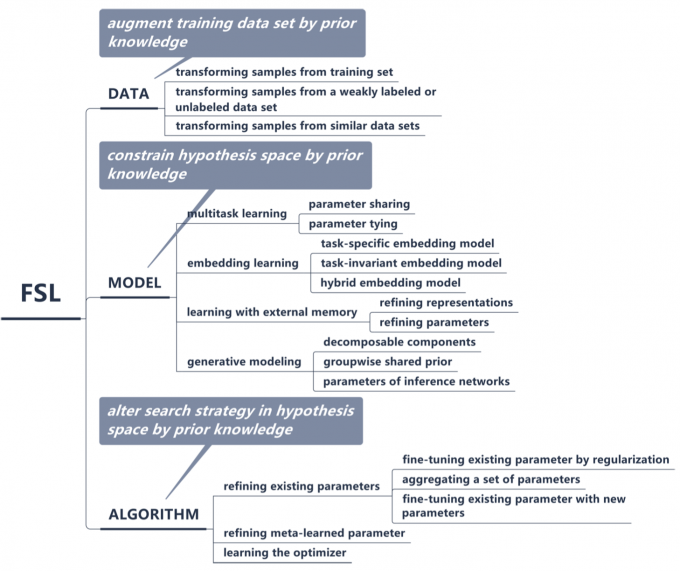
小样本学习的方法主要可以被归为三个方面：数据，模型，以及算法。其核心都是如何更好地利用先验知识。

从数据入手，主要是利用先验知识产生更大数量的数据；从模型入手，主要思想是利用先验知识来限制假设空间的大小，从而更快的找到最优点；从算法入手，主要思想是利用先验知识来改变搜索策略。

Data

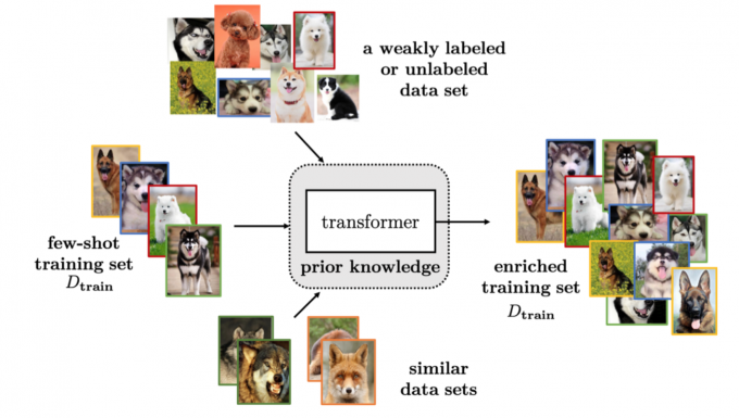
通过数据增强小样本的方法不改变搜索空间的大小，而是通过产生数据来帮助找到最优参数。它可以被归类为以下三种方法：

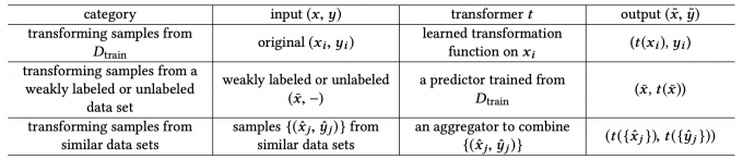
1. Transforming Samples from \(D_{train}\)
   该类方法通过对原训练数据的操作（如图像领域中的翻转等）进行数据增强，从而达到扩充数据的效果。
2. Transforming Samples from a Weakly Labeled or Unlabeled Data Set
   该类方法利用从训练数据中学习到的predictor对无监督或者弱监督的数据集进行标注，从而获得更大规模的数据集。
3. Transforming Samples from Similar Data Sets
   该类方法从一个相似且更大规模的数据集上迁移input-output pairs，aggregation weight通常基于样本间的相似性。

Model

Main idea: Use prior knowledge to constrain the complexity of ℋ, which results in a much smaller hypothesis space \(\widetilde{H}\).

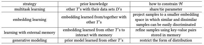
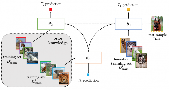
Multitask Learning

Multitask learning learns multiple related tasks simultaneously by exploiting both task-generic and task-specific information.

Given \(C\) related tasks \(T_1,…,T_C\), each \(T_c\) has a dataset\(D_c=\{D_{train}^c, D_{test}^c\}\).

The few-shot tasks are regarded as target tasks, and the rest as source tasks. Multitask learning learns from \(D_{train}^c\) to obtain \(\theta_c\) for train each \(T_c\).

Parameter Sharing

Parameter Sharing directly shares some parameters among tasks.

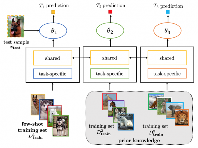
Parameter Tying

Parameter Tying encourages parameters of different tasks to be similar. A popular approach is by regularizing the \(\theta_c\).

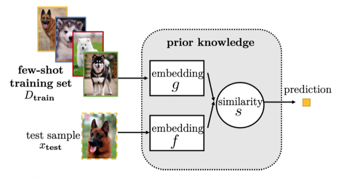
Embedding Learning

Embedding learning embeds each sample \(x_i \in \mathscr{X} \subseteq R^d\) to a lower-dimensional \(z_i \in \mathscr{Z} \subseteq R^m\).

It have three key components: - A function \(f\) which embeds test sample \(x_{test} \in D_test\) to \(\mathscr{Z}\) - A function \(g\) which embeds training sample \(x_{train} \in D_{train}\) to \(\mathscr{Z}\) - A similarity function \(s(·,·)\) which measures the similarity between \(f(x_{test})\) and \(g(x_I)\) in \(\mathscr{Z}\)

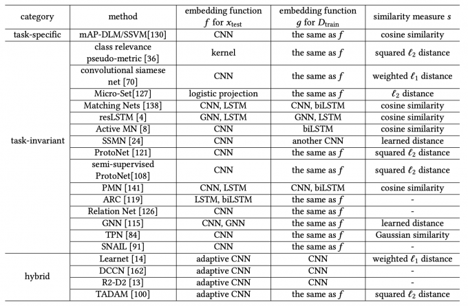
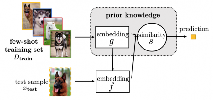
Task-specific embedding model

Learn an embedding function tailored for each task, by using only information from that task.

Task-invariant (i.e., general) embedding model

Learn a general embedding function from a large-scale data set containing sufficient samples with various outputs, and then directly use this on the new few-shot \(D_{train}\) without retraining.

E.g. Meta-learning (Matching Nets, Prototypical Networks, etc.), Siamese Net, etc.

Hybrid embedding model (encodes both task-specific and task-invariant information)

Learn a function which takes information extracted from \(D_{train}\) as input and returns an embedding which acts as the parameter for \(f(·)\) .

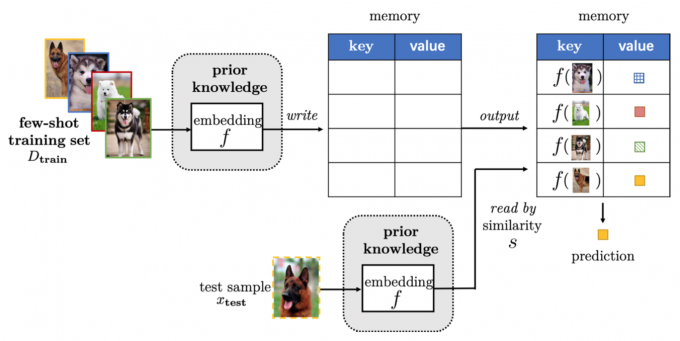
Learning with External Memory

Learning with external memory extracts knowledge from \(D_{train}\), and stores it in an external memory. Each new sample \(D_{test}\) is then represented by a weighted average of contents extracted from the memory.

A key-value memory is usually used in FSL.
Let the memory be \(M \in R^{(b \times m)}\), with each of its \(b\) memory slots \(M(i) \in R^m\) consisting of a key-value pair \(M(i)=(M_{key}(i),M_{value}(i))\).
A test sample \(x_{test}\) is first embedded by an embedding function \(f\), and used to query for the similar memory slots.

According to the functionality of the memory, it can be subdivided into two types. 1. Refining Representations
Put \(x_{train}\) into the memory, such that the stored key-value pairs can represent \(x_{test}\) more accurately. 2. Refining Parameters
Use a memory to parameterize the embedding function \(g(·)\) for a new \(x_{test}\) or classification model.

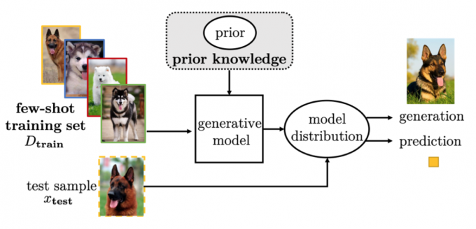
Generative Modeling

Generative modeling methods estimate the probability distribution \(p(x)\) from the observed \(x_i\) with the help of prior knowledge.

The observed \(x\) is assumed to be drawn from some distribution \(p(x;\theta)\) parameterized by \(\theta\).
Usually, there exists a latent variable \(z \backsim p(z;\gamma)\), so that \(x \backsim \int p(x|z;\theta)p(z;\gamma)dz\).
The prior distribution \(p(z;\gamma)\) brings in prior knowledge.

According to what the latent variable 𝑧 represents, it can be grouped into three types. 1. Decomposable Components
Samples may share some smaller decomposable components with samples from the other tasks. One then only needs to find the correct combination of these decomposable components, and decides which target class this combination belongs to. 2. Groupwise Shared Prior
Similar tasks have similar prior probabilities, and this can be utilized. 3. Parameters of Inference Networks
To find the best \(\theta\), one has to maximize the posterior

\[p(z|x;\theta,\gamma)=\frac{p(x,z;\theta ,\gamma)}{p(x;\gamma)}=\frac{p(x|z;\theta)p(z;\gamma)}{\int p(x|z;\theta)p(z;\gamma)dz}\]

Summary

1. Multitask learning
   Scenarios: Existing similar tasks or auxiliary tasks.
   Limitations: Joint training of all the tasks together is required. Thus, when a new few-shot task arrives, the whole multitask model has to be trained again.

2. Embedding learning
   Scenarios: A large-scale data set containing sufficient samples of various classes is available.
   Limitations: May not work well when the few-shot task is not closely related to the other tasks.

3. Learning with External Memory
   Scenarios: A memory network is available.
   Limitations: Incurs additional space and computational costs, which increase with memory size.

4. Generative modeling
   Scenarios: Performing tasks such as generation and reconstruction.
   Limitations: High inference cost, and more difficult to derive than deterministic models.

ALGORITHM

The algorithm is the strategy to search in the hypothesis space \(H\) for the parameter \(\theta\) of the best hypothesis \(h^*\).

Methods in this section use prior knowledge to influence how \(\theta\) is obtained, either by: 1. providing a good initialized parameter \(\theta_0\) 2. directly learning an optimizer to output search steps

In terms of how the search strategy is affected by prior knowledge, the methods can be classified into three groups.

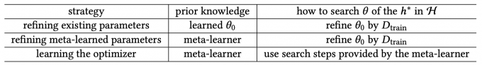
Refining Existing Parameters

Refining existing parameters: An initial \(\theta_0\) learned from other tasks, and is then refined using \(D_{train}\) .
The assumption is that \(\theta_0\) captures some general structures of the large-scale data. Therefore, it can be adapted to \(D\) with a few iterations.

Given the few-shot \(D_{train}\) , simply fine-tuning \(\theta_0\) by gradient descent may lead to overfitting. Hence, methods fine-tune \(\theta_0\) by regularization to prevent overfitting. They can be grouped as follows:

1. Early-stopping .
   It requires separating a validation set from D train to monitor the training procedure. Learning is stopped when there is no performance improvement on the validation set.
2. Selectively updating \(\theta_0\) .
   Only a portion of \(\theta_0\) is updated in order to avoid overfitting.
3. Updating related parts of \(\theta_0\) together.
   One can group elements of \(\theta_0\) (such as the neurons in a deep neural network), and update each group jointly with the same update information.
4. Using a model regression network.
   A model regression network captures the task-agnostic transformation which maps the parameter values obtained by training on a few examples to the parameter values that will be obtained by training on a lot of samples.

Aggregating a Set of Parameters

Sometimes, we do not have a suitable \(\theta_0\) to start with. Instead, we have many models that are learned from related tasks.

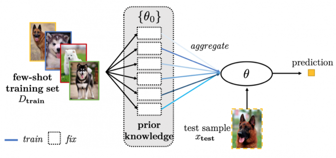
Instead of using the augmented data directly, the following methods use models (with parameters \(\theta_0\)’s) pre-trained from these data sets. The problem is then how to adapt them efficiently to the new task using \(D_{train}\) .

1. Unlabeled data set.
   One can pre-train functions from the unlabeled data to cluster and separate samples well. A neural network is then used to adapt them to the new task with the few-shot \(D_{train}\).
2. Similar data sets.
   few-shot object classification can be performed by leveraging samples and classifiers from similar classes. First, it replaces the features of samples from these similar classes by features from the new class. The learned classifier is then reused, and only the classification threshold is adjusted for the new class.

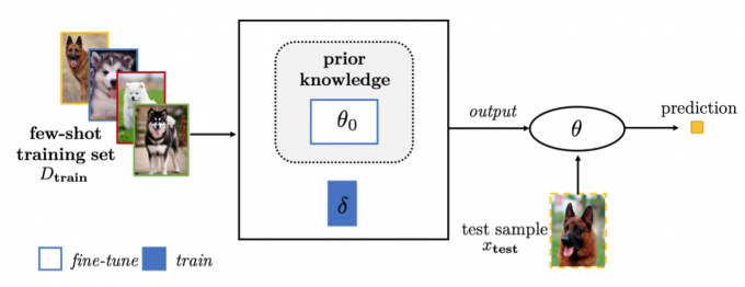
Fine-Tuning Existing Parameter with New Parameters

The pre-trained \(\theta_0\) may not be enough to encode the new FSL task completely. Hence, an additional parameter(s) \(\delta\) is used to take the specialty of D train into account. Specifically, this strategy expands the model parameter to become \(\theta = \{\theta_0,\delta\}\), and fine-tunes \(\theta_0\) while learning \(\delta\).

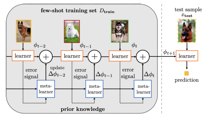
Refining meta-learned parameters

Methods in this section use meta-learning to refine the meta-learned parameter \(\theta_0\).The \(\theta_0\) is continuously optimized by the meta-learner according to performance of the learner.

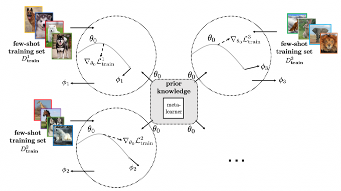
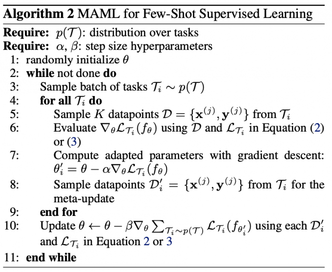
The meta-learned \(\theta_0\) is often refined by gradient descent. A representative method is the ModelAgnostic Meta-Learning (MAML).

Recently, many improvements have been proposed for MAML, mainly along the following three aspects:

1. Incorporating task-specific information.
   MAML provides the same initialization for all tasks. However, this neglects task-specific information, and is appropriate only when the set of tasks are all very similar.
2. Modeling the uncertainty of using a meta-learned \(\theta_0\).
   The ability to measure this uncertainty provides hints for active learning and further data collection . There are works that consider uncertainty for the meta-learned \(\theta_0\), uncertainty for the task-specific \(\phi_s\), and uncertainty for class n’s class-specific parameter\(\phi_{s,n}\).
3. Improving the refining procedure.
   Refinement by a few gradient descent steps may not be reliable. Regularization can be used to correct the descent direction.

Learning the optimizer

Instead of using gradient descent, methods in this section learns an optimizer which can directly output the update (\(\sum_{i=1}^t\Delta\theta^{i-1}\)). There is then no need to tune the stepsize \(\alpha\) or find the search direction, as the learning algorithm does that automatically.